Explaining the Discrepancies Between Hausfather et al. (2019) and Lewis&Curry (2018)

Reposted from Dr. Judith Curry’s Local weather And many others.

through Ross McKitrick

Difficult the declare that an enormous set of local weather mannequin runs revealed since 1970’s are in line with observations for the best causes.

Advent

Zeke Hausfather et al. (2019) (herein ZH19) tested a big set of local weather mannequin runs revealed because the 1970s and claimed they have been in line with observations, as soon as mistakes within the emission projections are thought to be. It is an engaging and precious paper and has gained a large number of press consideration. On this submit, I will be able to give an explanation for what the authors did after which speak about a few problems bobbing up, starting with IPCC over-estimation of CO2 emissions, a literature to which Hausfather et al. make a putting contribution. I will be able to then provide a critique of a few facets in their regression analyses. I in finding that they have got no longer specified their primary regression appropriately, and this undermines a few of their conclusions. The use of a extra legitimate regression mannequin is helping give an explanation for why their findings aren’t inconsistent with Lewis and Curry (2018) which did display fashions to be inconsistent with observations.

Define of the ZH19 Research:

A local weather mannequin projection can also be factored into two portions: the implied (brief) local weather sensitivity (to greater forcing) over the projection length and the projected building up in forcing. The primary derives from the mannequin’s Equilibrium Local weather Sensitivity (ECS) and the sea warmth uptake charge. It’ll be roughly equivalent to the mannequin’s brief local weather reaction (TCR), even though the dialogue in ZH19 is for a shorter length than the 70 years used for TCR computation. The second one comes from a submodel that takes annual GHG emissions and different anthropogenic elements as inputs, generates implied CO2 and different GHG concentrations, then converts them into forcings, expressed in Watts in line with sq. meter. The emission forecasts are in keeping with socioeconomic projections and are due to this fact exterior to the local weather mannequin.

ZH19 ask whether or not local weather fashions have overstated warming after we alter for mistakes in the second one issue because of inaccurate emission projections. So it’s necessarily a learn about of local weather mannequin sensitivities. Their conclusion, that fashions through and massive generate correct forcing-adjusted forecasts, signifies that fashions have usually had legitimate TCR ranges. However this conflicts with different proof (comparable to Lewis and Curry 2018) that CMIP5 fashions have overly excessive TCR values in comparison to observationally-constrained estimates. This discrepancy wishes rationalization.

One attention-grabbing contribution of the ZH19 paper is their tabulation of the 1970s-era local weather mannequin ECS values. The wording within the ZH19 Complement, which possibly displays that within the underlying papers, doesn’t distinguish between ECS and TCR in those early fashions. The reported early ECS values are:

• Manabe and Weatherald (1967) / Manabe (1970) / Mitchell (1970): 2.3K
• Benson (1970) / Sawyer (1972) / Broecker (1975): 2.4K
• Rasool and Schneider (1971) zero.8K
• Nordhaus (1977): 2.0K

If those in point of fact are ECS values they’re beautiful low through trendy requirements. It’s widely-known that the 1979 Charney File proposed a best-estimate vary for ECS of 1.five—four.5K. The follow-up Nationwide Academy record in 1983 through Nierenberg et al. famous (p. 2) “The local weather file of the previous hundred years and our estimates of CO2 adjustments over that length counsel that values within the decrease part of this vary are extra possible.” So the ones numbers may well be indicative of common considering within the 1970s. Hansen’s 1981 mannequin thought to be a spread of conceivable ECS values from 1.2K to a few.5K, selecting 2.8K for his or her most well-liked estimate, thus presaging the following use of usually upper ECS values.

However it’s not simple to inform if those are supposed to be ECS or TCR values. The latter are all the time not up to ECS, because of sluggish adjustment through the oceans. Type TCR values within the 2.zero–2.four Ok vary would correspond to ECS values within the higher part of the Charney vary.

If the fashions have excessive period ECS values, the truth that ZH19 in finding they keep within the ballpark of noticed floor reasonable warming, as soon as adjusted for forcing mistakes, suggests it’s a case of being proper for the mistaken reason why. The 1970s have been surprisingly chilly, and there may be proof that multidecadal interior variability used to be an important contributor to sped up warming from the overdue 1970s to the 2008 (see DelSole et al. 2011). If the fashions didn’t account for that, as a substitute attributing the whole lot to CO2 warming, it could require excessively excessive ECS to yield a fit to observations.

With the ones initial issues in thoughts, listed here are my feedback on ZH19.

There are some math mistakes within the writeup.

The principle textual content of the paper describes the method solely usually phrases. The web SI supplies statistical main points together with some mathematical equations. Sadly, they’re unsuitable and contradictory in puts. Additionally, the written method doesn’t appear to compare the web Python code. I don’t assume any essential effects hold on those issues, nevertheless it way studying and replication is unnecessarily tricky. I wrote Zeke about those problems prior to Christmas and he has promised to make any important corrections to the writeup.

One of the crucial outstanding findings of this learn about is buried within the on-line appendix as Determine S4, appearing previous projection levels for CO2 concentrations as opposed to observations:

Be mindful that, since there were few emission aid insurance policies in position traditionally (and none these days that bind on the international degree), the heavy black line is successfully the Industry-as-Same old series. But the IPCC again and again refers to its excessive finish projections as “Industry-as-Same old” and the low finish as policy-constrained. The truth is the excessive finish is fictional exaggerated nonsense.

I feel this graph must were in the principle frame of the paper. It presentations:

• Within the 1970s, fashions (blue) had a large unfold however on reasonable encompassed the observations (regardless that they cross in the course of the decrease part of the unfold);
• Within the 1980s there used to be nonetheless a large unfold however now the observations hug the ground of it, aside from for the horizontal line which used to be Hansen’s 1988 State of affairs C;
• Because the 1990s the IPCC repeatedly overstated emission paths and, much more so, CO2 concentrations through presenting a spread of long term eventualities, solely the minimal of which used to be ever lifelike.

I first were given curious about the issue of exaggerated IPCC emission forecasts in 2002 when the top-end of the IPCC warming projections jumped from about three.five levels within the 1995 SAR to six levels within the 2001 TAR. I wrote an op-ed within the Nationwide Put up and the Fraser Discussion board (each to be had right here) which defined that this variation didn’t end result from a metamorphosis in local weather mannequin behaviour however from using the brand new high-end SRES eventualities, and that many local weather modelers and economists thought to be them unrealistic. The in particular egregious A1FI situation used to be inserted into the combo close to the tip of the IPCC procedure in keeping with executive (no longer instructional) reviewer calls for. IPCC Vice-Chair Martin Manning distanced himself from it on the time in a widely-circulated e-mail, declaring that lots of his colleagues seen it as “unrealistically excessive.”

Some longstanding readers of Local weather And many others. may additionally recall the Castles-Henderson critique which got here out right now. It concerned with IPCC misuse of Buying Energy Parity aggregation regulations throughout international locations. The impact of the mistake used to be to magnify the relative source of revenue variations between wealthy and deficient international locations, resulting in inflated higher finish expansion assumptions for deficient international locations to converge on wealthy ones. Terence Corcoran of the Nationwide Put up revealed an editorial on November 27 2002 quoting John Reilly, an economist at MIT, who had tested the IPCC situation method and concluded it used to be “personally, a type of insult to science” and the process used to be “lunacy.”

Years later (2012-13) I revealed two instructional articles (to be had right here) in economics journals critiquing the IPCC SRES eventualities. Even if international general CO2 emissions have grown relatively somewhat since 1970, little of that is because of greater reasonable in line with capita emissions (that have solely grown from about 1.zero to one.four tonnes C in line with particular person), as a substitute it’s basically pushed through international inhabitants expansion, which is slowing down. The high-end IPCC eventualities have been in keeping with assumptions that inhabitants and in line with capita emissions would each develop hastily, the latter attaining 2 tonnes in line with capita through 2020 and over three tonnes in line with capita through 2050. We confirmed that the higher part of the SRES distribution used to be statistically very unbelievable as a result of it could require unexpected and sustained will increase in in line with capita emissions that have been inconsistent with noticed tendencies. In a follow-up article, my scholar Joel Wooden and I confirmed that the excessive eventualities have been inconsistent with the best way international power markets constrain hydrocarbon intake expansion. Extra just lately Justin Ritchie and Hadi Dowladabadi have explored the problem from a distinct attitude, particularly the technical and geological constraints that save you coal use from rising in the best way assumed through the IPCC (see right here and right here).

IPCC reliance on exaggerated eventualities is again within the information, because of Roger Pielke Jr.’s fresh column at the topic (in conjunction with a large number of tweets from him attacking the lifestyles and utilization of RCP8.five) and some other fresh piece through Andrew Montford. What is particularly egregious is that many authors are the use of the peak finish of the situation vary as “business-as-usual”, even after, as proven within the ZH19 graph, now we have had 30 years wherein business-as-usual has tracked the ground finish of the variety.

In December 2019 I submitted my evaluation feedback for the IPCC AR6 WG2 chapters. Many draft passages in AR6 proceed to confer with RCP8.five because the BAU result. That is, as has been mentioned prior to, lunacy—some other “insult to science”.

Apples-to-apples style comparisons calls for elimination of Pinatubo and ENSO results

The model-observational comparisons of number one hobby are the reasonably trendy ones, particularly eventualities A—C in Hansen (1988) and the central projections from quite a lot of IPCC stories: FAR (1990), SAR (1995), TAR (2001), AR4 (2007) and AR5 (2013). Because the comparability makes use of annual averages within the out-of-sample period the latter two time spans are too quick to yield significant comparisons.

Prior to analyzing the implied sensitivity ratings, ZH19 provide easy style comparisons. In lots of circumstances they paintings with a spread of temperatures and forcings however I will be able to center of attention at the central (or “Highest”) values to stay this dialogue transient.

ZH19 in finding that Hansen 1988-A and 1988-B considerably overstate tendencies, however no longer the others. Alternatively, I in finding FAR does as smartly. SAR and TAR don’t however their forecast tendencies are very low.

The principle forecast period of hobby is from 1988 to 2017. It’s shorter for the later IPCC stories because the get started yr advances. To make style comparisons significant, for the aim of the Hansen (1988-2017) and FAR (1990-2017) period comparisons, the 1992 (Mount Pinatubo) match must be got rid of because it depressed noticed temperatures however isn’t simulated in local weather fashions on a forecast foundation. Likewise with El Nino occasions. By way of no longer taking out those occasions the noticed style is overstated for the aim of comparability with fashions.

To regulate for this I took the Cowtan-Manner temperature sequence from the ZH19 information archive, which for simplicity I will be able to use because the lone observational sequence, and filtered out volcanic and El Nino results as follows. I took the IPCC AR5 volcanic forcing sequence (as up to date through Nic Lewis for Lewis&Curry 2018), and the NCEP pressure-based ENSO index (from right here). I regressed Cowtan-Manner on those two sequence and acquired the residuals, which I denote as “Cowtan-Manner adj” within the following Determine (notice each sequence are shifted to start out at zero.zero in 1988):

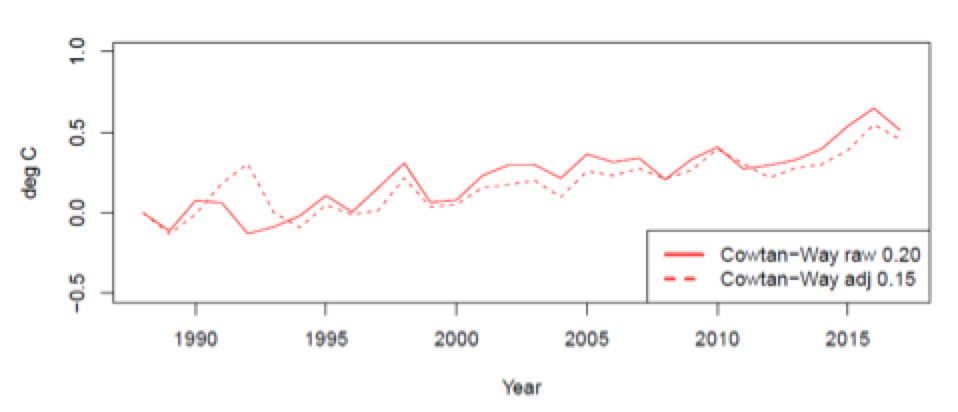
The tendencies, in Ok/decade, are indicated within the legend. The 2 style coefficients don’t seem to be considerably other from every different (the use of the Vogelsang-Franses check). Putting off the volcanic forcing and El Nino results reasons the rage to drop from zero.20 to zero.15 Ok/decade. The impact is minimum on periods that get started after 1995. Within the SAR subsample (1995-2017) the rage stays unchanged at zero.19 Ok/decade and within the TAR subsample (2001-2017) the rage will increase from zero.17 to zero.18 Ok/decade.

Here’s what the adjusted Cowtan-Manner information seems like, in comparison to the Hansen 1988 sequence:

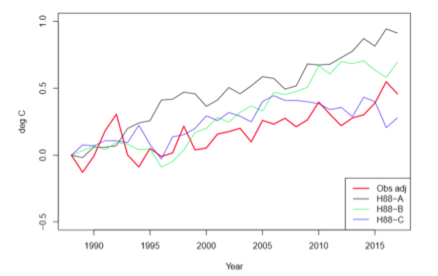
The linear style within the crimson line (adjusted observations) is zero.15 C/decade, just a little above H88-C (zero.12 C/decade) however smartly beneath the H88-A and H88-B tendencies (zero.30 and zero.28 C/decade respectively)

The ZH19 style comparability method is an advert hoc mixture of OLS and AR1 estimation. Because the method write-up is incoherent and their manner is non-standard I received’t attempt to reflect their self belief periods (my OLS style coefficients fit theirs then again). As an alternative I’ll use the Vogelsang-Franses (VF) autocorrelation-robust style comparability method from the econometrics literature. I computed tendencies and 95% CI’s within the two CW sequence, the three Hansen 1988 A,B,C sequence and the primary 3 IPCC out-of-sample sequence (denoted FAR, SAR and TAR). The consequences are as follows:

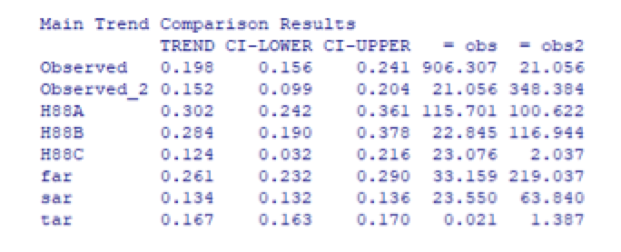
The OLS tendencies (in Ok/decade) are within the 1^st column and the decrease and higher bounds at the 95% self belief periods are within the subsequent two columns.

The four^th and five^th columns record VF check ratings, for which the 95% essential worth is 41.53. Within the first two rows, the diagonal entries (906.307 and 348.384) are exams on a null speculation of no style; each reject at extraordinarily small importance ranges (indicating the tendencies are vital). The off-diagonal ratings (21.056) check if the tendencies within the uncooked and changed sequence are considerably other. It does no longer reject at five%.

The entries within the next rows check if the rage in that row (e.g. H88-A) equals the rage in, respectively, the uncooked and changed sequence (i.e. obs and obs2), after adjusting the pattern to have equivalent time spans. If the ranking exceeds 41.53 the check rejects, that means the tendencies are considerably other.

The Hansen 1988-A style forecast considerably exceeds that during each the uncooked and changed noticed sequence. The Hansen 1988-B forecast style does no longer considerably exceed that within the uncooked CW sequence nevertheless it does considerably exceed that within the adjusted CW (because the VF ranking rises to 116.944, which exceeds the 95% essential worth of 41.53). The Hansen 1988-C forecast isn’t considerably other from both noticed sequence. Therefore, the one Hansen 1988 forecast that fits the noticed style, as soon as the volcanic and El Nino results are got rid of, is situation C, which assumes no building up in forcing after 2000. The post-1998 slowdown in noticed warming finally ends up matching a mannequin situation wherein no building up in forcing happens, however does no longer fit both situation wherein forcing is authorized to extend, which is attention-grabbing.

The forecast tendencies in FAR and SAR don’t seem to be considerably other from the uncooked Cowtan-Manner tendencies however they do vary from the adjusted Cowtan-Manner tendencies. (The FAR style additionally rejects in opposition to the uncooked sequence if we use GISTEMP, HadCRUT4 or NOAA). The discrepancy between FAR and observations is because of the projected style being too huge. Within the SAR case, the projected style is smaller than the noticed style over the similar period (zero.13 as opposed to zero.19). The adjusted style is equal to the uncooked style however the sequence has much less variance, which is why the VF ranking will increase. When it comes to CW and Berkeley it rises sufficient to reject the rage equivalence null; if we use GISTEMP, HadCRUT4 or NOAA neither uncooked nor adjusted tendencies reject in opposition to the SAR style.

The TAR forecast for 2001-2017 (zero.167 Ok/decade) by no means rejects in opposition to observations.

So as to summarize, ZH19 pass in the course of the workout of evaluating forecast to noticed tendencies and, for the Hansen 1988 and IPCC tendencies, maximum forecasts don’t considerably vary from observations. However a few of that obvious have compatibility is because of the 1992 Mount Pinatubo eruption and the series of El Nino occasions. Putting off the ones, the Hansen 1988-A and B projections considerably exceed observations whilst the Hansen 1988 C situation does no longer. The IPCC FAR forecast considerably overshoots observations and the IPCC SAR considerably undershoots them.

To be able to refine the model-observation comparability it is usually very important to regulate for mistakes in forcing, which is the following activity ZH19 adopt.

Implied TCR regressions: a specification problem

ZH19 outline an implied Temporary Local weather Reaction (TCR) as

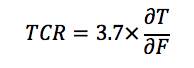
the place T is temperature, F is anthropogenic forcing, and the by-product is computed because the least squares slope coefficient from regressing temperature on forcing over the years. Suppressing the consistent time period the regression for mannequin i is solely

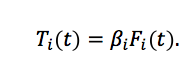
The TCR for mannequin i is due to this fact the place three.7 (W/m²) is the assumed equilibrium CO2 doubling coefficient. They in finding 14 of the 17 implied TCR’s are in line with an observational counterpart, outlined because the slope coefficient from regressing temperatures on an observationally-constrained forcing sequence.

In regards to the post-1988 cohort, sadly ZH19 depended on an ARIMA(1,zero,zero) regression specification, or in different phrases a linear regression with AR1 mistakes. Whilst the temperature sequence they use are most commonly style desk bound (i.e. desk bound after de-trending), their forcing sequence don’t seem to be. They’re what we name in econometrics built-in of order 1, or I(1), particularly the primary variations are style desk bound however the ranges are nonstationary. I will be able to provide an excessively transient dialogue of this however I will be able to save the longer model for a magazine article (or a proper touch upon ZH19).

There’s a huge and rising literature in econometrics journals in this factor because it applies to local weather information, with plenty of competing effects to plow through. At the time spans of the ZH19 information units, the usual exams I ran (particularly Augmented Dickey-Fuller) point out temperatures are trend-stationary whilst forcings are nonstationary. Temperatures due to this fact can’t be a easy linear serve as of forcings, in a different way they’d inherit the I(1) construction of the forcing variables. The use of an I(1) variable in a linear regression with out modeling the nonstationary element correctly can yield spurious effects. Because of this this can be a misspecification to regress temperatures on forcings (see Phase four.three in this bankruptcy for a partial rationalization of why that is so).

How must any such regression be carried out? A while sequence analysts are seeking to unravel this catch 22 situation through claiming that temperatures are I(1). I will be able to’t reflect this discovering on any information set I’ve noticed, but when it seems to be true it has huge implications together with rendering maximum kinds of style estimation and research hitherto meaningless.

I feel it’s much more likely that temperatures are I(zero), as are herbal forcings, and anthropogenic forcings are I(1). However this creates a large downside for time sequence attribution modeling. It way you’ll’t regress temperature on forcings the best way ZH19 did; if truth be told it’s no longer glaring what the proper manner can be. One conceivable strategy to continue is named the Toda-Yamamoto manner, however it’s only usable when the lags of the explanatory variable can also be incorporated, and on this case they are able to’t as a result of they’re completely collinear with every different. The principle different choice is to regress the primary variations of temperatures on first variations of forcings, so I(zero) variables are on either side of the equation. This might suggest an ARIMA(zero,1,zero) specification quite than ARIMA(1,zero,zero).

However this wipes out a large number of data within the information. I did this for the later fashions in ZH19, regressing every one’s temperature sequence on every one’s forcing enter sequence, the use of a regression of Cowtan-Manner at the IPCC general anthropogenic forcing sequence as an observational counterpart. The use of an ARIMA(zero,1,zero) specification aside from for AR4 (for which ARIMA(1,zero,zero) is indicated) yields the next TCR estimates:

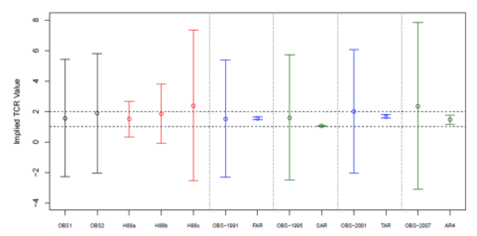
The comparability of hobby is OBS1 and OBS2 to the H88a—c effects, and for every IPCC record the OBS-(startyear) sequence in comparison to the corresponding model-based worth. I used the unadjusted Cowtan-Manner sequence because the observational opposite numbers for FAR and after.

In a single sense I reproduce the ZH19 findings that the mannequin TCR estimates don’t considerably vary from noticed, on account of the overlapping spans of the 95% self belief periods. However that’s no longer very significant because the 95% observational CI’s additionally surround zero, adverse values, and implausibly excessive values. Additionally they surround the Lewis & Curry (2018) effects. Necessarily, what the effects display is that those information sequence are too quick and volatile to supply legitimate estimates of TCR. The actual distinction between fashions and observations is that the IPCC fashions are too strong and constrained. The Hansen 1988 effects in truth display a extra lifelike uncertainty profile, however the TCR’s vary so much a few of the 3 of them (level estimates 1.five, 1.nine and a pair of.four respectively) and for 2 of the 3 they’re statistically insignificant. And naturally they overshoot the noticed warming.

The illusion of actual TCR estimates in ZH19 is spurious because of their use of ARIMA(1,zero,zero) with a nonstationary explanatory variable. An issue with my means this is that the ARIMA(zero,1,zero) specification doesn’t make environment friendly use of data within the information about doable longer term or lagged results between forcings and temperatures, if they’re provide. However with such quick information samples it’s not conceivable to estimate extra advanced fashions, and the I(zero)/I(1) mismatch between forcings and temperatures rule out discovering a easy manner of doing the estimation.

Conclusion

The obvious inconsistency between ZH19 and research like Lewis & Curry 2018 that experience discovered observationally-constrained ECS to be low in comparison to modeled values disappears as soon as the regression specification factor is addressed. The ZH19 information samples are too quick to supply legitimate TCR values and their regression mannequin is laid out in any such manner that it’s prone to spurious precision. So I don’t assume their paper is informative as an exercize in local weather mannequin analysis.

It’s, then again, informative on the subject of previous IPCC emission/focus projections and presentations that the IPCC has for a very long time been depending on exaggerated forecasts of worldwide greenhouse fuel emissions.

I’m thankful to Nic Lewis for his feedback on an previous draft.

Remark from Nic Lewis

Those early fashions solely allowed for will increase in forcing from CO2, no longer from all forcing brokers. Since 1970, general forcing (in line with IPCC AR5 estimates) has grown greater than 50% sooner than CO2-only forcing, so if early mannequin temperature tendencies and CO2 focus tendencies over their projection sessions are consistent with noticed warming and CO2 focus tendencies, their TCR values should were greater than 50% above that implied through observations.